Intro

This project aims to compare how effectively Scala and Python implementations of an ALS movie recommender can be accelerated using GPUs with Spark on a cloud-computing platform. We use Spark MLlib to build the Python and Scala recommenders, and we use the NVIDIA spark-rapids package to integrate an AWS EMR cluster with GPUs. We also compare the speedup between a cluster utilizing GPUs and one with only CPUs. Lastly, we compare how well the equivalent Scala and Python implementations perform on the MovieLens datasets of 100k movie ratings, 1M movie ratings, and 20M movie ratings and 25M movie ratings to measure weak scaling.

Problem Definition

Background to Recommender Systems

Recommender systems address the problem of information overload (Ullman, 2010). Unlike physical retailers, online outlets have a ‘long-tail’ of esoteric items and therefore cannot show the full range to users because they would be overwhelmed. This has led to the rise of recommender systems, which show only a subset of items to users based on a prediction of what the user wants. The huge number of items (whether it be information, goods or services) that online outlets provide requires large-scale parallel computation so that an appropriate subset of items can be offered to users in a reasonable timeframe.

The rise of recommender systems also brings about the question of algorithmic accountability. The increasing use of neural network recommender systems may mean a greater opacity to how recommendations are made and why they make particular recommendations. Therefore, it is important that systems such as collaborative filtering (which is presented in this project) can provide a viable alternative to neural network recommender systems in the interests of interpretability. It is easier to explore how and why collaborative filtering recommenders make recommendations. Therefore, optimising the efficiency, speed and training of collaborative filtering recommenders is an important task.

Implicit vs Explicit Recommender Systems

Many recommender systems are based on implicit data. For example, in order to recommend pages for an editor to correct on wikipedia, the recommender might use implicit information about how many times a page has been edited in the past.

Explicit recommender systems are based on explicit ratings data where a user has deliberately rated items. Although this data is ostensibly more ‘intentional,’ the ratings are often very sparse in comparison to implicit data. This means that the recommender will have to predict many separate data points. This further reinforces the importance of a parallel computing infrastructure for this project.

Content-based Filtering

A technique mainly used in the early days of recommender systems, content-based filtering uses item features to recommend other items similar to what the user likes, based on their previous actions or explicit feedback. While the model can make recommendations solely from a single user’s data, this approach struggles when recommending outside the users’ main interests. It also requires a fair amount of hand-engineering the feature representation of the items to produce a good model, and is typically slower to train than other approaches.

Collaborative Filtering

Collaborative filtering has been a popular method of designing recommender systems, especially since the Netflix Prize in 2009 (Koren, 2009). At the heart of collaborative filtering is the idea that the preferences of one user can be modelled based on information from the preferences of other users by calculating the rating similarity between users.

Alternating Least Squares (ALS)

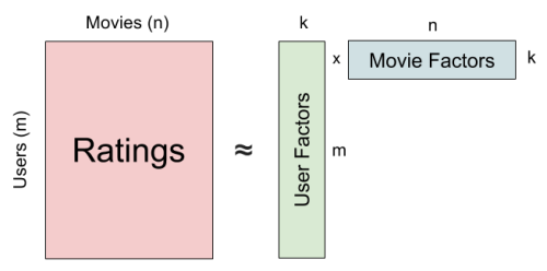
In our application, the sparsity and the high dimensionality of the ratings data cause a problem when finding similarities between users. Thus collaborative filtering recommenders rely on matrix factorization to reduce the sparsity and the dimensions of the ratings matrix. In this project, we explore the Alternating Least Square (ALS) matrix factorization algorithm. Compared to other matrix factorization algorithms such as Stochastic Gradient Descent, ALS is easier to parallelize and requires less iterations to reach a good result. The ALS algorithm decomposes the rating matrix A into 2 matrices, W (user factors) and H (movie factors). A user’s rating on a movie will be encoded into latent features in these 2 factored matrices. The idea behind this is that if a user gives good ratings to Avengers, Wonder Woman and Iron Man, these 3 ratings should not be regarded as 3 separate preferences, but a general opinion that the user likes superhero movies.

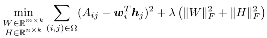
The objective of the ALS algorithm is to minimize the least squares error of the ratings as well as the regularizations (Yu et. al., 2013).

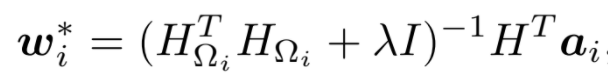
W and H are updated separately by fixing one and updating the other. Below is the updating step for a row in W.

The complexity of ALS is

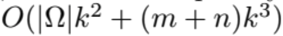
, where Ω is the set of indices for observed ratings. For updating each row of W or H, we need quadratic time to compute the H^T*H in the updating step, and cubic time to solve the least squares. Thus we have the overall complexity in this form. Though ALS has higher complexity per iteration than some other matrix factorization algorithms, it’s parallelizability, less iteration requirement to achieve good factorization results, and implementation in Spark MLlib make it easy to scale up the dataset.

Big Data and Compute Requirements

The datasets used include up to 25 million movie recommendations, and therefore ALS matrix factorization can take a long time to run. As mentioned above, if collaborative filtering is to be a viable (and potentially more interpretable) alternative to neural network-based recommenders, it is important that this application can be scaled to large datasets and perform ALS matrix factorization quickly. Indeed, as users can come join a platform/application very fast, it is critical that any recommender system used at scale would have the capacity to quickly compute user preferences.

A second critical reason that it is important to explore high-end data analytics and big compute solutions for ALS matrix factorization is that, although matrix factorization is highly parallelizable, a large body of research suggests that it does not scale well to large datasets (Yu et. al., 2013). ALS can theoretically be easily parallelized iteratively because each of the rows (W and H) can be updated individually, which is outlined above; however, it may not be possible to fit the entirety of row W and H on a node, which limits the potential to parallelize these operations at large scale.

How our work relates to wider research

There has been much work on parallelizing recommender systems, including parallelizing ALS. Similarly, there has been work on the differences between Scala and Python for use with Spark. However, according to our literature review, there has been little work done to compare how Scala and Python perform on different GPU configurations, and even less on specifically comparing the parallel performance of Spark and Scala implementations of an ALS movie recommender. Therefore, our project draws on both of these bodies of work and aims to add an additional element by exploring the differences between Python and Scala implementations of a parallelized movie recommender using Spark.

Python versus Scala

There is some academic work testing the speedup differences between Scala and Python, and within industry it is widely regarded that Scala can achieve a large speedup compared to Python on many tasks. The name ‘Scala’ originally comes from it’s prime function, which is to scale to large quantities of data. Therefore, it’s origins are different than Python, which is a more general-purpose language. Scala is also the native language of Spark, and therefore it may not be surprising that Scala is thought to be faster than Python. Specifically, research points to several reasons that Scala programs with Spark can be faster than PySpark programs. First, Scala is statically typed, not dynamically typed like Python, which means the type of variable is known at compile time in Scala programmes (Ghandi, 2018). This is practical because it means the programmer should be able to catch bugs quicker in Scala than Python, where variables are only known at runtime. It also means that there is additional time spent at runtime understanding the variables in Python, which is not the case with Scala.

Possibly the most important reason that Scala runs Spark programs faster than Pyspark is the fact that it uses the Java Virtual Machine (JVM). This means that Scala is able to communicate much more effectively with Hadoop, whereas python does not work as well with Hadoop services. There is also evidence to suggest that Scala’s primitives allow it to perform well on programs involving executing several tasks at the same time (Ghandi, 2018).

ALS and Recommender Systems

There has been significant academic work exploring the parallelisation of recommender systems. Though Stochastic Gradient Descent (SGD) is a faster way to optimize this problem, it is not parallelizable (Yu et. al., 2013). Researchers have proposed alternatives to both ALS and SGD, such as Fast Parallel Stochastic Gradient Descent (FPSG) and CCD++. The CCD++ algorithm was specifically developed to address the fact that ALS does not scale particularly well to large datasets because of the nature of the complexity mentioned above, where there is cubic time complexity for the target rank.

One research paper on parallelising ALS matrix factorisation using a GPU compared to CPU found that the use of GPUs resulted in significant overhead, though they observed that the impact of GPUs was greater for larger datasets compared to smaller datasets (Siomos, 2016).

Experimental Design and Solution

Dataset

MovieLens datasets are a series of stable benchmark datasets created by GroupLens Research over the past two decades (Harper & Konstan, 2015). One of the reasons we wanted to use this dataset is because it is widely used in research on recommender systems and parallelizing Matrix Factorization (Yu et. al., 2013). Therefore, they are easily replicable by other researchers and can be compared to other recommender system results (e.g. Dooms et. al. 2014; Qiu, 2016; Siomos, 2018).

Some of the new MovieLens datasets include tag genome data with relevance scores. However, we do not use this data for our recommender. The attributes that we use in order to utilize ALS to compute the preferences of users are ‘userId’, ‘rating’ and ‘movieId’.

Size

For all datasets we preprocessed the files to remove the header and any columns other than ‘userId’, ‘rating’ and ‘movieId’ because these were not relevant for the recommender; specifically, we removed the ‘timestamp’ column as it caused errors when trying to run the Scala script. For comparing GPU and CPU clusters, we used the MovieLens 20M ratings dataset; it was released in 2015 and updated in 2016.

For measuring the recommenders on different dataset sizes we vary the size of the dataset between 100k, 1M, 20M and 25M. They have the following characteristics:

• MovieLens 100K (2.3 MB): 100,000 ratings from 1000 users on 1700 movies
• MovieLens 1M dataset (12 MB): 1 million ratings from 6000 users on 4000 movies
• MovieLens 20M dataset (305.2 MB): 20 million ratings on 27,000 movies by 138,000 users
• MovieLens 25M dataset (390.2 MB): 25 million ratings on 62,000 movies by 162,000 users.

Distribute ALS Matrix Factorization: MLlib and Parallelization

MLlib is Apache Spark’s machine learning library, which made it an easy decision to use for our solution. MLlib can be easily integrated with a cluster and EC2 instances, and it is a Spark Library.

The central scalability problem, as outlined above, is not the parallelization of ALS as such, but the parallelization of ALS with large scale data. When the rows that need to be iterated over are very large, the task of distributing the data becomes much more difficult. A central reason for using MLlib is to address this challenge through a principled approach. Indeed, there are multiple aspects of the design of MLlib that allow effective implementation of distributed ALS matrix factorisation on large datasets. ‘Hybrid partitioning’ is used to decrease the amount of shuffling that happens at each iteration, and ‘block-to-block join’ effectively distributes the user and item matrices across nodes so that you can also decrease the amount of overhead from partitioning (Das et. al., 2016). Specifically, matrices are partitioned into in-blocks and out-blocks in a way such that the parts of each matrice needed for each iteration is accessible.

Both the Scala and Python recommenders use MLlib and are very similar. This was a purposeful decision because we wanted to compare the two recommenders and therefore wanted to make them as similar as possible. It was also important to use the same Spark library (MLlib) for both.

Accelerating Our Application

The first idea we got for creating a recommender system that utilized GPUs on a Spark cluster came from the CS 205 Spring 2019 project titled Parallelized Amazon Recommendation System Based on Spark and OpenMP. In their Suggested Improvements section, they mentioned utilizing GPU instances to try and further facilitate parallelism of their application. After doing some research, we found that while Spark was first created in 2009 and the introduction of AWS with GPU instances began in November 2010, it hasn’t been until the past few years that people have begun using GPU instances on Spark. One of the big reasons for this increased interest is the rise of data science, and the recognition that data analytics and machine learning can benefit from GPU acceleration to minimize execution time. With the introduction of RAPIDs.AI from NVIDIA that offered CUDA-integrated software tools in October 2018, it became the first platform to offer GPU capabilities for a data science workflow. One branch of the larger RAPIDS open source software libraries and APIs is the RAPIDS Accelerator for Apache Spark, which leverages the power of the RAPIDS cuDF library and the scale of the Spark distributed computing framework. After looking at the incredible performance and cost benefits posted on the spark-rapids homepage and recognizing that very few people have examined using the combination of Spark and GPUs, we wanted to see for ourselves if we may be able to replicate some of these performance speedups for our recommender system using ALS. We also wanted to utilize AWS on which to integrate the GPUs with Spark since it is the most widely used cloud-computing platform, and as well as due to our familiarity with its ecosystem through our continued work on it over the course of this semester.

How to Replicate our Code

Setting up a spark-rapids Cluster with GPU

GPU Cluster Details:

• Release label: emr-6.2.0
• Hadoop distribution: Amazon 3.2.1
• Applications:Spark 3.0.1, Livy 0.7.0, JupyterEnterpriseGateway 2.1.0
• Master: m5.xlarge, 4 vCore, 16 GiB memory, EBS Storage:64 GiB
• Core: g4dn.2xlarge, 8 vCore, 32 GiB memory, 225 SSD GB storage
• Task: g4dn.2xlarge, 8 vCore, 32 GiB memory, 225 SSD GB storage

Software and Configuration

1. Go to AWS EMR.
2. Select ‘create cluster’.
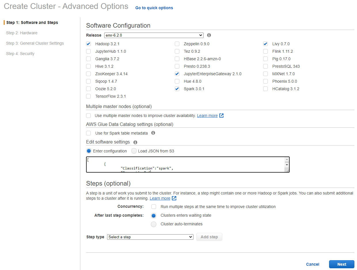
3. Select ‘Advanced Options’.
4. Select emr-6.2.0 for release and ‘Hadoop 3.2.1, Spark 3.0.1, Livy 0.7.0 and JupyterEnterpriseGateway 2.1.0’ for software options.
5. In the “Edit software settings” field enter the following configuration: Note that spark.task.resource.gpu.amount is set to 1/(number of cores per executor) which allows us to run parallel tasks on the GPU. Therefore, as we dynamically change the number of cores per executor we will also have to change this using the command line.

{

[
	{
		"Classification":"spark",
		"Properties":{
			"enableSparkRapids":"true"
		}
	},
	{
		"Classification":"yarn-site",
		"Properties":{
			"yarn.nodemanager.resource-plugins":"yarn.io/gpu",
			"yarn.resource-types":"yarn.io/gpu",
			"yarn.nodemanager.resource-plugins.gpu.allowed-gpu-devices":"auto",
			"yarn.nodemanager.resource-plugins.gpu.path-to-discovery-executables":"/usr/bin",
			"yarn.nodemanager.linux-container-executor.cgroups.mount":"true",
			"yarn.nodemanager.linux-container-executor.cgroups.mount-path":"/sys/fs/cgroup",
			"yarn.nodemanager.linux-container-executor.cgroups.hierarchy":"yarn",
			"yarn.nodemanager.container-executor.class":"org.apache.hadoop.yarn.server.nodemanager.LinuxContainerExecutor"
		}
	},
	{
		"Classification":"container-executor",
		"Properties":{
			
		},
		"Configurations":[
			{
				"Classification":"gpu",
				"Properties":{
					"module.enabled":"true"
				}
			},
			{
				"Classification":"cgroups",
				"Properties":{
					"root":"/sys/fs/cgroup",
					"yarn-hierarchy":"yarn"
				}
			}
		]
	},
	{
        "Classification":"spark-defaults",
        "Properties":{
        "spark.plugins":"com.nvidia.spark.SQLPlugin",
        "spark.sql.sources.useV1SourceList":"",
        "spark.executor.resource.gpu.discoveryScript":"/usr/lib/spark/scripts/gpu/getGpusResources.sh",
        "spark.submit.pyFiles":"/usr/lib/spark/jars/xgboost4j-spark_3.0-1.0.0-0.2.0.jar",
        "spark.executor.extraLibraryPath":"/usr/local/cuda/targets/x86_64-linux/lib:/usr/local/cuda/extras/CUPTI/lib64:/usr/local/cuda/compat/lib:/usr/local/cuda/lib:/usr/local/cuda/lib64:/usr/lib/hadoop/lib/native:/usr/lib/hadoop-lzo/lib/native:/docker/usr/lib/hadoop/lib/native:/docker/usr/lib/hadoop-lzo/lib/native",
        "spark.rapids.sql.concurrentGpuTasks":"2",
        "spark.executor.resource.gpu.amount":"1",
        "spark.executor.cores":"12",
        "spark.task.cpus ":"1",
        "spark.task.resource.gpu.amount":"0.125",
        "spark.rapids.memory.pinnedPool.size":"2G",
        "spark.executor.memoryOverhead":"2G",
        "spark.locality.wait":"0s",
        "spark.sql.shuffle.partitions":"200",
        "spark.sql.files.maxPartitionBytes":"256m",
        "spark.sql.adaptive.enabled":"false"
        }
	},
	{
		"Classification":"capacity-scheduler",
		"Properties":{
			"yarn.scheduler.capacity.resource-calculator":"org.apache.hadoop.yarn.util.resource.DominantResourceCalculator"
		}
	}
]

}

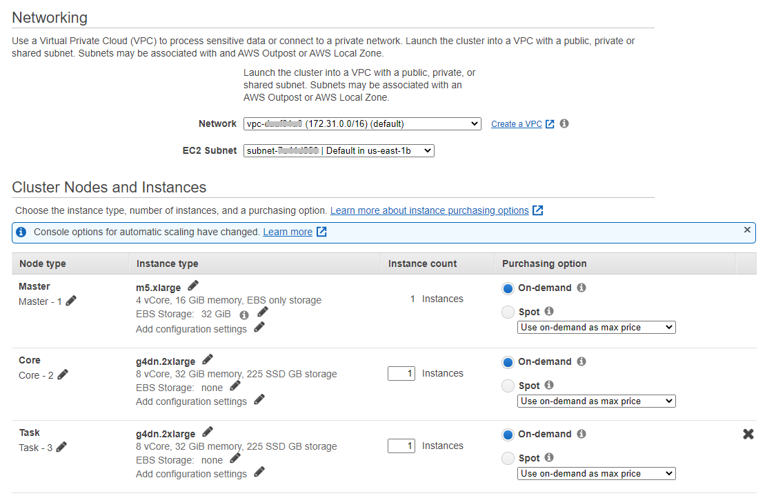
1. Select the default network and subnet.
2. Change the instance type to g4dn.2xlarge. Select one core and one task instance.

General Cluster Settings

1. Add a cluster name and an S3 bucket to write cluster logs to.

2. Add a custom ‘Bootstrap Actions’ to allow cgroup permissions to YARN on the cluster. You can use the script at this S3 bucket: s3://recommender-s3-bucket/bootstrap.json

   Alternatively, you could use the script below in your own s3 bucket:

	#!/bin/bash
 
  	set -ex
 
  	sudo chmod a+rwx -R /sys/fs/cgroup/cpu,cpuacct
  	sudo chmod a+rwx -R /sys/fs/cgroup/devices
	

Security Settings

1. Select an EC2 key pair.
2. In the “EC2 security groups” tab, confirm that the security group chosen for the “Master” node allows for SSH access. Follow these instructions to allow inbound SSH traffic if the security group does not allow it yet.
3. Select ‘Create Cluster’ and SSH into the Master Node of the Cluster.

See Spark-Rapids documentation for further details

Setting up a CPU Cluster

CPU Cluster Details:

• Release label: emr-6.2.0
• Hadoop distribution: Amazon 3.2.1
• Applications: Spark 3.0.1, Zeppelin 0.9.0
• Master and Core: m4.2xlarge: 32 GiB of memory, 8 vCPUs, EBS-only, 64-bit platform

1. Go to AWS EMR.
2. Select ‘create cluster’.
3. Select emr-6.2.0 for release and “Spark” for application, which has Spark 3.0.1, Hadoop 3.2.1.
4. Select m4.2xlarge as instance type, and 3 instances (1 master and 2 core nodes).
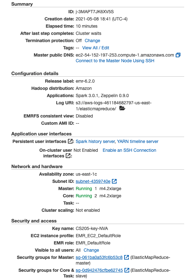
5. Choose a cluster name and your key pair. Leave everything else default. Create cluster.
6. Check the summary page is similar to the below image.
7. Go to EC2 -> Instances, find your master node instance, and confirm that the security group chosen for the “Master” node allows for SSH access. Follow these instructions to allow inbound SSH traffic if the security group does not allow it yet.
8. SSH into the Master Node of the Cluster

Scripts

Link to Repository

There were two main scripts utilized for this project: recommender.py and recommender.scala. As mentioned previously, the scripts were purposely made to be as similar as possible to best compare execution times. Both scripts contain the variable names and documentation except for where the language syntax differs, and are heavily drawn from the Apache Spark MLlib examples repository (Scala and Python). The high-level overview of the script is as follows: create a SparkContext, read in the .csv file, map the dataset to an RDD in the form required for the ALS() function, train the ALS on the RDD, make predictions based on the user-movie tuple, and compare the true user-movie ratings with the predicted user-movie ratings from the ALS using mean squared error. We recognize that a more robust ALS prediction model can be made which contains a train-test split, but our focus for this project was execution time comparisons; therefore, we were content as long as each script produced similar mean squared errors (within 0.05) depending on the dataset used.

Two other scripts created for this project were the build.sbt used for the GPU, and the build.sbt used for the CPU. The extension .sbt stands for Simple Build Tool, and it is an open-source build tool for Scala and Java projects that allows for easily compiling and creating .jar files for projects. The build.sbt file contains metadata information about the project, as well as all dependencies that are required to run the code. Originally, we had to create two different versions due to different Scala versions on the two different clusters (GPU had Scala version 2.12.10 available, while CPU had Scala version 2.11.12 available), but fortuantely were able to update the CPU cluster to have the same Spark and Scala version as the GPU cluster.

Challenges of MLlib, spark-rapids, and Scala

There were multiple challenges we faced throughout the course of this project. An initial difficulty was finding an application that would allow us to easily utilize Spark with GPUs on an AWS cluster. Our initial approach was to use the IBM GPU Enabler package which integrated with Spark, but it was a dormant library that hadn’t been updated since April 2018 and did not provide information about use on AWS. We also had concerns about spark-rapids being used with Scala (as outlined shortly), but after some testing we were able to figure it out. While spark-rapids did have a very well-detailed and documented start-up guide for RAPIDS on an AWS EMR cluster, there were many different configuration options that needed to be understood. Fortunately, we recognized that the “spark.executor.cores” and the “spark.task.resource.gpu.amount” were the two arguments that must be tuned in order to produce results with different numbers of executors.

The largest bottleneck for us actually occurred when creating the .jar file that is needed to run a Scala script. While there were many tutorials on how to do this (e.g. here and here, and here), none proved particularly effective in walking us through how to create a .sbt file that could be properly compiled to create a .jar file that could then be executed. One of our hopes with this project is to actually create a Medium article that provides a step-by-step guide on how to easily create a Scala script using .sbt on an EMR cluster.

The next challenge was deciding on the hyperparameters for the ALS model since MLlib provided many different tuning options. In order for ALS matrix factorization to converge, it is important to iterate for fewer than 20 iterations. Secondly, it is also important to set the rank (the number of latent factors used to predict empty values in the user-item matrix) equal to or below 10.

Regarding the scripts, there was one particular spot that we could not exactly match the Python and Scala implementations. For the PySpark MLlib implementation, the function required a .predictAll() function when performing the prediction, while the Scala MLlib implementation provided a .predict() function. After examining the code it does not appear that the difference should cause any execution time changes as a result of the two different functions, but it is something we wanted to note since we could not reconcile this without changing a couple other parts of the Python or Scala script; this way we minimized potential differences.

A final bottleneck that was pervasive throughout the testing process was the cost for GPUs. A g4dn.2xlarge EC2 instance costs $0.752/hr for On-Demand pricing, so we did our best to be cognizant of our limited budget. However, each member unfortunately exceeded the $100 credit limit in order to produce the most comprehensive results to showcase our project.

Step-by-step guide for running Python script

Note: we recommend that you hard code the commands, instead of copy and paste them from the website.

1. From the GitHub repository, copy over the python script to the EMR cluster

   $ scp -i ~/.ssh/your_.pem_file_here python/recommender.py hadoop@your_Master_public_DNS_here:/home/hadoop

2. Log in to the EMR cluster again

   $ ssh -i ~/.ssh/your_.pem_file_here hadoop@your_Master_public_DNS_here

3. Now, upload the MovieLens dataset you want to use to the EMR cluster; for this example, we will upload the Movielens 20mL dataset

   If uploading the dataset from the public S3 bucket to the EMR cluster home repository

   $ aws s3 cp s3://als-recommender-data/data/ratings_20ml.csv .

4. Upload the dataset ratings_20ml.csv to the Hadoop file system

   When running the command $ hadoop fs -ls, you should see something similar to this: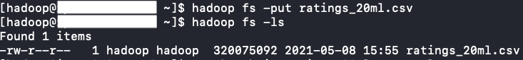

   

5. You should now be able to run the below code and see results

   spark-submit recommender.py ratings_20ml.csv

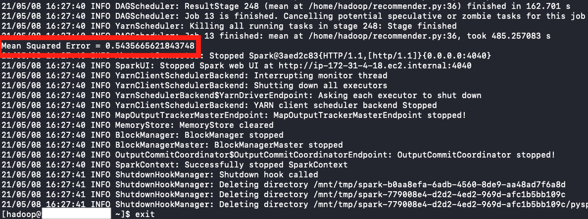
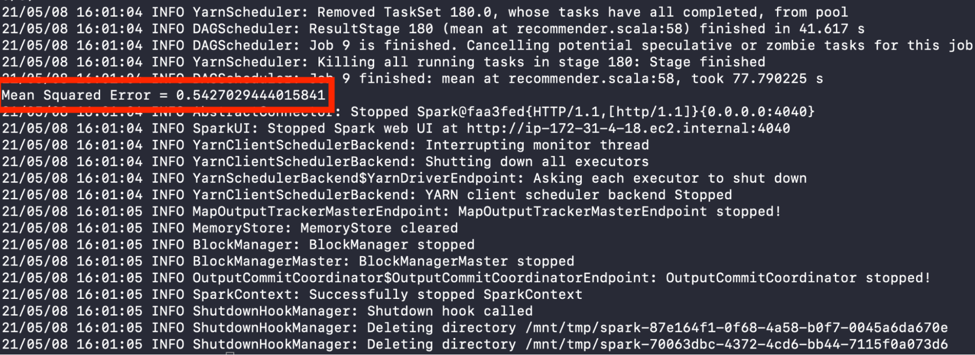
6. When the code has completed, you should be able to see the Mean Squared Error produced by the ALS PySpark Recommender

   

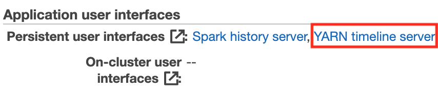
7. To profile the code and calculate execution time, from the Summary tab of your EMR cluster, click on YARN timeline server under the Application user interfaces section

   

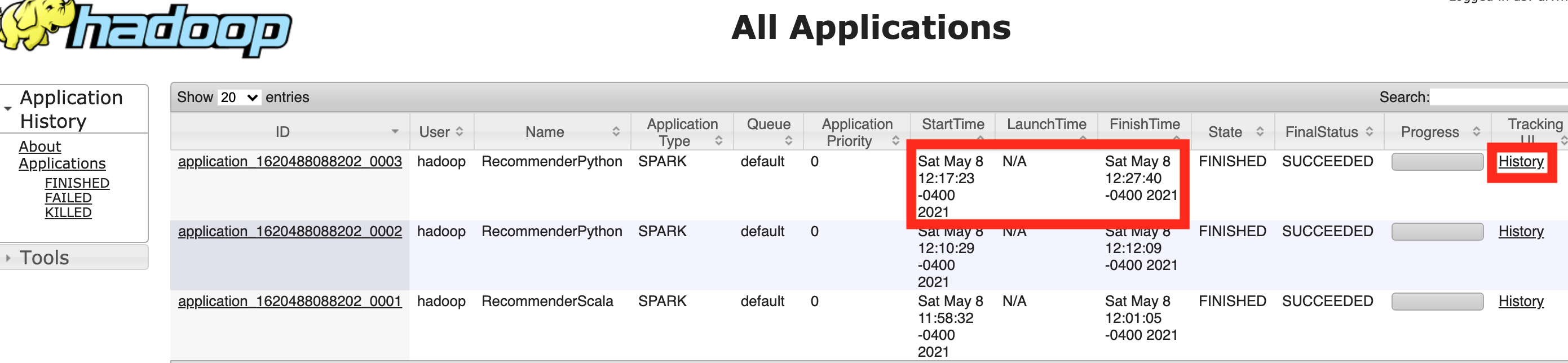
8. You can now calculate the execution time of the recommender system. We see that the script took 10 minutes 17 seconds to run (StartTime: Sat May 8 12:17:23 - FinishTime: Sat May 8 12:27:40). To profile the code, you can click on the History link under the Tracking UI column header.

   

9. We can now view how long each function call takes in order to run our script

   

step-by-step guide for running Scala script

Note: we recommend that you hard code the commands, instead of copy and paste them from the website.

While the setup for running a Python script on the EMR cluster is very straightforward, the process for running a Scala script requires a few more steps; however, as you’ll see shortly during the results section, it is well worth it.

These steps below are for running on the GPU cluster. The only difference for running on the CPU cluster is the folder imported in Step 1

1. From the GitHub repository, copy over the Scala script to the EMR cluster

   $ scp -i ~/.ssh/your_.pem_file_here scala_GPU/* hadoop@your_Master_public_DNS_here:/home/hadoop

   Please note that if you are trying to run this on the CPU cluster, perform this command instead:

   scp -i ~/.ssh/your_.pem_file scala_CPU/* hadoop@your_Master_public_DNS:/home/hadoop

2. Log in to the EMR cluster again

   $ ssh -i ~/.ssh/your_.pem_file_here hadoop@your_Master_public_DNS_here

3. Download sbt to the EMR cluster

   curl https://bintray.com/sbt/rpm/rpm | sudo tee /etc/yum.repos.d/bintray-sbt-rpm.repo

   sudo yum install sbt

4. Create the appropriate directory structure for the .sbt file to compile based on the Spark tutorial “Self Contained Applications” with Scala

   mkdir src; cd src; mkdir main; cd main; mkdir scala; cd scala; mv ../../../recommender.scala .; cd ~

5. Check that the directory structure contains at least this information when running the below command from the home directory of the EMR cluster

   find .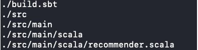

   

6. Run the command

   sbt package

   1. This compiles the recommender.scala project (in this case, the build.sbt and recommender.scala script) and packages it into a .jar (Java ARchive) file, which can then be executed by the Scala interpreter
   2. To make sure it has compiled successfully, you should see something similar to this

1. Now, upload the MovieLens dataset you want to use to the EMR cluster; for this example, we will upload the Movielens 20mL dataset

   If uploading the dataset from the public S3 bucket to the EMR cluster home repository

   $ aws s3 cp s3://als-recommender-data/data/ratings_20ml.csv .

2. Upload the dataset ratings_20ml.csv to the Hadoop file system

   When running the command $ hadoop fs -ls, you should see something similar to this:

   

3. You should now be able to run the below code and see results (please confirm the location and name of the .jar file is the same)

   spark-submit --class "RecommenderScala" target/scala-2.12/scala-recommender_2.12-1.0.jar ratings_20ml.csv

4. When the code has completed, you should be able to see the Mean Squared Error produced by the ALS Scala Recommender

Please see Steps 7-9 of step-by-step guide for running Python script for how to profile the code.

Results

Below are the results when using the CPU and GPU clusters on the 20M dataset for the Python and Scala recommender scripts

CPU Results (20M Dataset)

Python

Mean Squared Error	Execution Time (seconds)	Speedup	Python Command
0.543	721	N/A	spark-submit –num-executors 1 –executor-cores 1 recommender.py ratings_20ml.csv
0.544	571	1.26	spark-submit –num-executors 1 –executor-cores 2 recommender.py ratings_20ml.csv
0.542	561	1.28	spark-submit –num-executors 1 –executor-cores 4 recommender.py ratings_20ml.csv
0.543	482	1.49	spark-submit –num-executors 1 –executor-cores 8 recommender.py ratings_20ml.csv

Scala

Mean Squared Error	Execution Time (seconds)	Speedup	Scala Command
0.545	139	N/A	spark-submit –class “RecommenderScala” –num-executors 1 –executor-cores 1 target/scala-2.12/scala-recommender_2.12-1.0.jar ratings_20ml.csv
0.545	109	1.28	spark-submit –class “RecommenderScala” –num-executors 1 –executor-cores 2 target/scala-2.12/scala-recommender_2.12-1.0.jar ratings_20ml.csv
0.543	108	1.29	spark-submit –class “RecommenderScala” –num-executors 1 –executor-cores 4 target/scala-2.12/scala-recommender_2.12-1.0.jar ratings_20ml.csv
0.544	115	1.21	spark-submit –class “RecommenderScala” –num-executors 1 –executor-cores 8 target/scala-2.12/scala-recommender_2.12-1.0.jar ratings_20ml.csv

GPU Results (20M Dataset)

Python

Mean Squared Error	Execution Time (seconds)	Speedup	Python Command
0.543	961	N/A	spark-submit –executor-cores 1 –conf spark.task.resource.gpu.amount=1 recommender.py ratings_20ml.csv
0.545	554	1.73	spark-submit –executor-cores 2 –conf spark.task.resource.gpu.amount=0.5 recommender.py ratings_20ml.csv
0.545	503	1.91	spark-submit –executor-cores 4 –conf spark.task.resource.gpu.amount=0.25 recommender.py ratings_20ml.csv
0.545	704	1.37	spark-submit –executor-cores 8 –conf spark.task.resource.gpu.amount=0.125 recommender.py ratings_20ml.csv

Scala

Mean Squared Error	Execution Time (seconds)	Speedup	Scala Command
0.543	221	N/A	spark-submit –class “RecommenderScala” –executor-cores 1 –conf spark.task.resource.gpu.amount=1 target/scala-2.12/scala-recommender_2.12-1.0.jar ratings_20ml.csv
0.544	132	1.67	spark-submit –class “RecommenderScala” –executor-cores 2 –conf spark.task.resource.gpu.amount=0.5 target/scala-2.12/scala-recommender_2.12-1.0.jar ratings_20ml.csv
0.543	104	2.13	spark-submit –class “RecommenderScala” –executor-cores 4 –conf spark.task.resource.gpu.amount=0.25 target/scala-2.12/scala-recommender_2.12-1.0.jar ratings_20ml.csv
0.541	147	1.50	spark-submit –class “RecommenderScala” –executor-cores 8 –conf spark.task.resource.gpu.amount=0.125 target/scala-2.12/scala-recommender_2.12-1.0.jar ratings_20ml.csv ratings_20ml.csv

20M Dataset - GPU

Overall it does not seem that using a GPU provided as much speed-up as we expected. We can see that moving from one core (threads within the worker node) to two or four cores reduces the runtime for both Python and Scala programs. However, the runtime of both Python and Scala programs when using the GPU cluster increases from 4 to 8 cores. This is an especially pronounced increase for the Python implementation. One explanation for this is that moving from 4 to 8 cores leads to larger overheads, which outweigh the benefit of using a GPU to accelerate calculations, particularly for ALS matrix factorization. Indeed, based on profiling the code it appears that an additional bottleneck is the calculation of mean squared error. This requires the aggregation of values across data on multiple nodes and thus requires a high degree of communication overhead. It may be that, although the GPU effectively speeds up one part of the application (the ALS), it actually adds to the overheads in subsequently processing the resulting distributed outputs in order to calculate the mean squared error.

20M Dataset - CPU Results and comparison with GPU

We ran the Python and Scala implementations on GPU and CPU using 1 executor. We see that when the program is run serially with 1 thread, CPU is faster than GPU for both Scala and Python. If we look at the runtime comparison plots, using more cores does not decrease GPU execution time significantly against CPU execution time. This makes sense since the CPU consists of cores optimized for serial processing which perform well on a single task run on 1 executor and 1 core, while GPU consists of thousands of cores that are optimized for parallel computing of multiple tasks (Olena, 2018). We also see that Scala is significantly faster than Python, as we’ll discuss shortly.

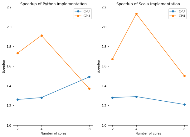
Now when looking at the speedup plots, we see that GPU has much higher speedup levels than CPU for 2 and 4 cores because of its suitability in parallelized tasks. When we reach 8 cores, the runtimes for GPU tend to become slower and the speedups decrease more drastically than CPU due to synchronization and GPU-CPU communication overhead. We also see the speedups for Python and Scala are very similar.

Example Scala and Python Recommender Runtimes

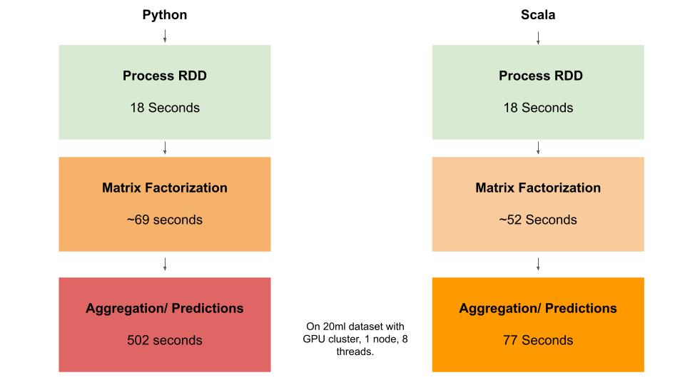
It is clear from the diagram above that a major bottleneck in both applications is the final step of the recommender, which involves aggregation and prediction. Although it appears that the matrix factorization operations are effectively distributed by MLlib in both applications, it seems that the major bottleneck is the calculation of predictions. Our results show that the ALS Matrix factorization element of our application scales relatively effectively to larger datasets (20M and 25M); however, the aggregation and prediction part of the application does not scale well. Our initial assumptions before testing were that ALS matrix factorisztion was the major bottleneck, and we did not consider there may be a second major bottleneck of aggregation of results that needes to be parallelized. This could explained by the fact that Scala uses the Java Virtual Machine and communicates with Hadoop natively, which may be particularly important in an aggregation task or any task where distributed data needs to be rapidly aggregated in order to perform calculations.

Throughput

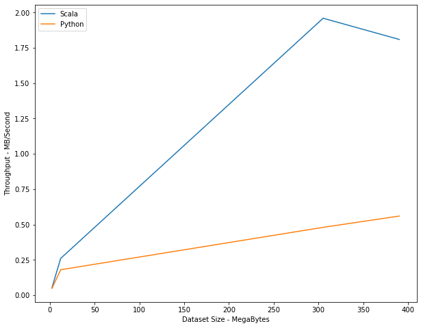
Scala is designed primarily to distribute data across nodes. Therefore, speedup is, in some senses, a byproduct of the primary goal of Spark, which is to scale effectively (in terms of cost and speed) as datasets get large. In general we would expect the throughput of data to scale as the dataset size increases. Indeed, we would expect Scala to scale better than Python, as this is Scala’s primary function.

We can see that the difference between Scala and Python is magnified as the datasets become larger. While the difference is less significant at the 3 MB level (the 100K dataset), it becomes very marked once we get to the 300+ MB level (the 20M dataset and 25M dataset). This suggests that the Scala implementation does indeed scale better in terms of throughput than the PySpark implementation. However, it is noticeable that the throughput declines from the 20M to 25M dataset. Thus it would be useful in future work to test whether this is a continuing decline by utilizing a larger dataset to observe if there is decreasing marginal scalability for the Scala implementation. One important point to note as well is that this decreasing scalability may be a result of the type of the application, as the fact that ALS Matrix Factorization does not scale well to large dataset sizes is widely observed in research. (Yu et. al., 2013)

Dataset Size	Python (runtime/ throughput)	Scala (runtime/ throughput)
100k (2.3 MB)	48 s, 0.048 MB/s	42 s, 0.054 MB/s
1M (12 MB)	66 s, 0.18 MB/s	47 s, 0.26 MB/s
20M (305.2 MB)	632 s, 0.48 MB/s	156 s, 1.96 MB/s
25M (390.2 MB)	691, 0.56 MB/s	216, 1.81 MB/s

Scala and the future of heterogeneous and specialised programming languages

In order to carry out this project, we had to use three new frameworks beyond our experience from CS205: Scala, NVIDIA spark-rapids and Spark MLlib. As mentioned previously, the most significant of these challenges was implementing both a Scala and Python version of the recommender. All of our team was new to Scala and therefore learning how to build an executable jar file was a prerequisite to our experiment. Fortunately, this challenge also gave us insight into the potential future evolution of programming languages. Although more heterogeneous hardware is increasingly being used for specialised problems, our project focused on this use of a specialist programming language for big data analytics: Scala. Our experience with the difficulty of using Scala points to the potential trade-off between the time it takes to learn a new programming language and paradigm compared to the potential performance benefits. In contrast, this trade-off may be very different for heterogeneous hardware.

A second challenge was utilising NVIDIA spark-rapids to accelerate the recommender with a GPU. Setting up the cluster using advanced settings on AWS, as well as understanding how to apportion sections of the GPUs available were both time-consuming and tedious. It is notable that spark-rapids is part of a wider NVIDIA ecosystem, which includes infrastructure to support Dask and other frameworks and infrastructure for machine learning. Specifically, it seems to be primarily designed for integration with Python, which may be why some aspects of the code are written in this language. Therefore, although Scala is the native language of Spark, it is notable that other frameworks that can be integrated with Spark, such as spark-rapids, are more geared towards PySpark, Pandas, and Scikit-learn users. This is a second reason to believe that the movement towards more specialised programming languages may be constrained. Our project suggests some reasons why the trend to heterogeneous hardware may be much stronger than the trend towards more heterogeneous programming languages and paradigms.

Conclusion

Based on our results, due to the large amount of distribution that is being performed under the hood with Spark and the additional communication/synchronization that is required when utilizing a GPU, we’ve found that a GPU with Spark may not be the most effective solution when trying to decrease the execution time for a ALS recommendation model. We have also idenfified that there is a trade-off with using Scala: it is more complex to operationalize and may involve taking time to learn new skills, but typically provides stronger performance. Even though Scala provides better speedup than Python, the aggregation and MSE calculation bottleneck in our program is still a problem for the Scala implementation, even though it is less of a bottleneck than in Python. Ultimately, Scala provides a powerful tool for data scientists, especially in scaling big data ALS matrix factorization applications. However, it is not a silver bullet for improving the performance of ALS matrix factorization, and therefore multiple factors should be taken into account when building the compute and data analytics solution to any ALS matrix factorization problem in future.

Next Steps

In order to verify whether the speed-up observed using the Scala recommender can be attributed to Scala’s use of the Java Virtual Machine it would be useful to also run the same experiment with a Java recommender. Indeed, Scala was originally designed to address perceived problems with Java for big data analytics; therefore, we might expect Scala to perform better than Java in other ways, and it would be useful to explore how they differ in more detail.

Second, it would be useful to further our understanding of the scalability of both the Python and Scala implementations by testing the recommenders on larger datasets. Specifically, we would have liked to generate a new dataset using fractal expansion and implement the recommenders on that dataset, but we were not able to implement this in the given time frame. Since it seems that the Scala throughput falls off slightly after the 20M dataset, it would be particularly useful to test the Scala recommenders on higher datasets and observe whether the perceived view that ALS recommenders cannot be effectively scaled to very large datasets is accurate.

Third, our working hypothesis about the bottleneck of our application at the aggregation and prediction stage is that this part of the application is not effectively parallelised here. Since both Python and Scala are higher level languages and Spark is a higher-level abstraction where the handling of the distribution is all under-the-hood, it would be beneficial to explore our theory in greater detail and see if this is potentially parallelizable.

Fourth, it would be interesting to see results when utilizing multiple CPUs/GPUs. Due mainly to budget constriants we were not able to horizontally scale our architecture in the way we would like, so future work would examine results when we add instances to the clusters.

Lastly, it would be useful to implement recommenders using dataframes rather than RDDs, as Spark plan to phase out RDDs and it is thought that the dataframe framework in Spark is faster than the RDD framework. This is also a feature designed to integrate seamlessly with widely used libraries, such as pandas, and therefore it would be interesting to explore whether the use of dataframes, rather than RDDs, would change the relationship between the Python and Scala speedups that we observed in this project.

References

Das, A., Xiangrui, M., Upadhyaya, I., Talwalkar, A. and Meng, X. (2016) ‘Collaborative Filtering as a Case-Study for Model Parallelism on Bulk Synchronous Systems.’, ACM.

Dooms et. al. 2014, ‘In-memory, distributed content-based recommender system’, Journal of Intelligent Information Systems 42.

Gandhi, P. (2018) ‘Apache Spark: Python vs. Scala’, KD.

Harper, F.M. & Konstan, J. A., (2015) ‘The MovieLens Datasets: History and Context’, ACM Transactions on Interactive Intelligent Systems

Koren, Y. The Belkor Solution to the Netflix Grand Prize

Olena (2018) GPU vs CPU Computing: What to choose?

Qiu, Y. (2016) ‘Recosystem: recommender system using parallel matrix factorization’

Siomos, T. (2016) ‘Parallel Implementation of Basic Recommendation Algorithms’ , International Hellenic University.

Ullman, J. D. et al, (2010) Mining of Massive Datasets: Chapter 9: Recommendation Systems, p321.

Yu et. al. (2013), ‘Parallel Matrix Factorization for Recommender Systems’, Knowledge and Information Systems.